
This is something that is tested almost every year in Grade 12 exam papers: the Subtotal command in the Outline group of the Data ribbon. It is a useful way to aggregate (summarise) large amounts of data quickly. Very important: this is the Subtotal feature, NOT the SUBTOTAL function! Download the Excel spreadsheet and follow along.
Scenario 1
In the first 2 scenarios, we have one year’s financial data. The data represents monthly sales figures. Each month belongs to a financial quarter (column A).
In the example, I use the Subtotal feature to create an outline of the data which includes totals for each of the quarters, as well as a total for the year.
Scenario 2
The second scenario uses the same data with a slightly different format: the monthly sales figures have been grouped into financial quarters (column A).

The Golden Rule is: “You must sort the data by the column on which you are going to group the data”.
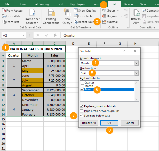
- Select the data, headings included (A2:C14)
- Activate the Data menu
- Click the Subtotal button
- Select the column by which you want to aggregate (group) the data — the data must be sorted by this column!
- Choose which function you want to use
- Choose which column of values you want to aggregate (calculate)
- Select the Summary below data option
- Click OK
- Your data now has subtotals for each Quarter
- You can expand and collapse the levels of the data outline